Tuning a PID Controller

Heat treatment processes exemplify the need for PID control. To ensure consistent product quality the temperature inside an oven or furnace must be kept within narrow limits. Any disturbance, such as when a product is added or withdrawn or a ramp function is applied, must be handled appropriately. Although simple in concept, the mathematics underpinning PID control is complex and achieving optimal performance entails selecting process-specific values for a range of interacting parameters.

The process of finding these values is referred to as “tuning.” When tuned optimally, a PID temperature controller minimizes deviation from the set point, and responds to disturbances or set point changes quickly but with minimal overshoot.

This White Paper from OMEGA Engineering discusses how to tune a PID controller. Even though many controllers provide auto tune capabilities, an understanding of PID tuning will help in achieving optimal performance. Individual sections address:

PID control is based on feedback. The output of a device or process, such as a heater, is measured and compared with the target or set point. If a difference is detected a correction is calculated and applied. The output is measured again and any required correction recalculated.

PID stands for proportional-integral-derivative. Not every controller uses all three of these mathematical functions. Many processes can be handled to an acceptable level with just the proportional-integral terms. However, fine control, and especially overshoot avoidance, requires the addition of derivative control.

In proportional control the correction factor is determined by the size of the difference between set point and measured value. The problem with this is that as the difference approaches zero, so too does the correction, with the result that the error never goes to zero.

The integral function addresses this by considering the cumulative value of the error. The longer the set point-to-actualvalue difference persists the greater the size of correction factor calculated. However, when there is a delay in response to the correction this leads to an overshoot and possibly oscillation about the set point. Avoiding this is the purpose of the derivative function. This looks at the rate of change being achieved, progressively modifying the correction factor to lessen its effect as the set point is approached.

Every process has unique characteristics, even when the equipment is essentially identical. Airflow around ovens will vary, ambient temperatures will alter fluid density and viscosity, and barometric pressure will change from hour to hour. The PID settings (principally the gain applied to the correction factor along with the time used in the integral and derivative calculations, termed “reset” and “rate”) must be selected to suit these local differences.

In broad terms, there are three approaches to determining the optimal combination of these settings: manual tuning, tuning heuristics, and automated methods.

With enough information about the process being controlled, it may be possible to calculate optimal values of gain, reset and rate. Often the process is too complex, but with some knowledge, particularly about the speed with which it responds to error corrections, it is possible to achieve a rudimentary level of tuning.

Manual tuning is done by setting the reset time to its maximum value and the rate to zero and increasing the gain until the loop oscillates at a constant amplitude. (When the response to an error correction occurs quickly a larger gain can be used. If response is slow a relatively small gain is desirable). Then set the gain to half of that value and adjust the reset time so it corrects for any offset within an acceptable period. Finally, increase the rate until overshoot is minimized.

Many rules have evolved over the years to address the question of how to tune a PID loop. Probably the first, and certainly the best known, are the Zeigler-Nichols (ZN) rules.

First published in 1942, Zeigler and Nichols described two methods of tuning a PID loop. These work by applying a step change to the system and observing the resulting response. The first method entails measuring the lag or delay in response and then the time taken to reach the new output value. The second depends on establishing the period of a steady-state oscillation. In both methods these values are then entered into a table to derive values for gain, reset time and rate.

ZN is not without issues. In some applications it produces a response considered too aggressive in terms of overshoot and oscillation. Another drawback is that it can be time-consuming in processes that react only slowly. For these reasons some control practitioners prefer other rules such as Tyreus-Luyben or Rivera, Morari and Skogestad.

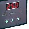
Most process controllers sold today incorporate auto-tuning functions. Operating details vary between manufacturers but all follow rules similar to those described above. Essentially, the controller “learns” how the process responds to a disturbance or change in set point, and calculates appropriate PID settings. In the case of a temperature controller like OMEGA’s CNi8 series, when “Auto Tune” is selected the controller activates an output. By observing both the delay and rate with which the change is made it calculates optimal P, I and D settings, which can then be fine-tuned manually if needed. (Note that this controller requires the set point to be at least 10°C above the current process value for auto tuning to be performed).

Newer and more sophisticated controllers, such as OMEGA’s Platinum series of temperature and process controllers, incorporate fuzzy logic with their auto tune capabilities. This provides a way of dealing with imprecision and nonlinearity in complex control situations, such as are often encountered in manufacturing and process industries, and helps with tuning optimization.

Ovens and furnaces used in industrial heat treatment are required to achieve consistent results regardless of how the mass and humidity of material being heated may vary. This makes such equipment ideal for PID control. Pumps used for moving fluids are a similar application, where variation in media properties could change system outputs unless an effective feedback loop is implemented.

Motion control systems also use a form of PID control. However, as the response is orders of magnitude faster than the systems described above these require a different form of controller to that discussed here.

PID control is used to manage many processes. Correction factors are calculated by comparing the output value to the set point and applying gains that minimize overshoot and oscillation while effecting the change as quickly as possible.

PID tuning entails establishing appropriate gain values for the process being controlled. While this can be done manually or by means of control heuristics, most modern controllers provide auto tune capabilities. However, it remains important for control professionals to understand what happens after the button in pressed.